Linear Regression Using Solver
Linear regression creates a statistical model that can be used to predict the value of a dependent variable based on the value(s) of one more independent variables.
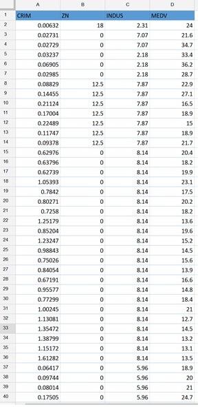
The example dataset below was taken from the well-known Boston housing dataset. The information in this dataset was gathered by the US Census Bureau from census tracts within the Boston area. Each of the features (or variables) describes a characteristic impacting the selling price of a house.

To run a linear regression:
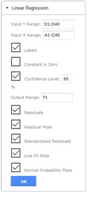
- On the XLMiner Analysis ToolPak pane, click Linear Regression
- Enter D1:D40 for "Input Y Range". This is the output variable.
- Enter A1:C40 for "Input X Range". These are the predictor variables.
- Keep "Labels" selected since the first row contains labels describing the contents of each column.
- If "Constant is Zero" is selected, there will be no constant term in the equation. Leave this option unchecked for this example.
- Select "Confidence Level 95%".
- Enter F1 for the "Output Range".
- Select "Residuals" to display the unstandardized residuals in the output. Unstandardized residuals are computed by the formula: Unstandardized residual = Actual response – Predicted response.
- Select "Residual Plots" to display the Residual Plots for each variable.
- Select "Standardized" under Residuals to display the standardized residuals in the output. Standardized residuals are obtained by dividing the unstandardized residuals by their respective standard deviations.
- Select "Line Fit Plots" to display the Line Fit Plots for each variable.
- Select "Normal Probability Plots" to display the Normal Probability Plot for the Y variable.
- Click OK.

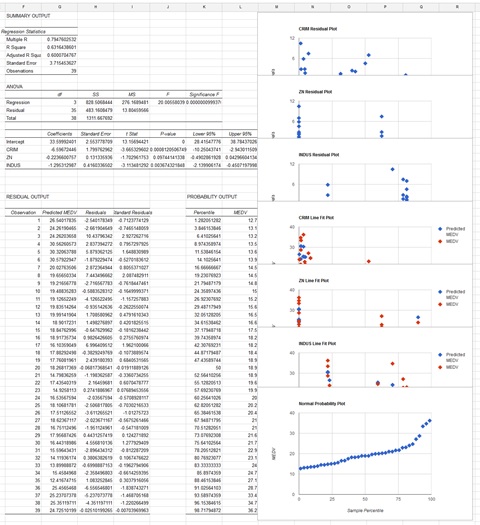
The results are below.

Using these results, the regression model can be written as: Median Value of Owner Occupied Home = 33.6 – 6.597 * CRIM - .2237 * ZN -1.295 * INDUS. For a more detailed explanation of these results, see any standard statistics reference text.
